Calculating transfer functions of effective systems
Sometimes it is useful to simulate a simpler effective thermo-optomechanical system that
emulates a more complex physical one, but that is not strictly physical itself. In such
cases it may be difficult to simulate the DC fields needed to describe this effective
system. In Finesse, the DC fields are known as the carrier_solution. Usually when
calculating a FrequencyResponse, the DC fields are first computed and
then used in the computation of the AC response. It is also possible to override this DC
calculation by providing a carrier_solution where the DC fields have been manually
set to their desired values. We illustrate this here with the effective three mirror
coupled cavity, which describes some of the dynamics of modern and future gravitational
wave detectors.
Warning
It is your responsibility to ensure that sensible DC fields are being set. Finesse
will happily return garbage if you haven’t been careful when providing a
carrier_solution to one of the FrequencyResponse actions.
You can manually provide a carrier_solution to any of the four
FrequencyResponse actions, but we’ll demonstrate it here only with
FrequencyResponse.
The DARM coupled cavity
The optical topology used by all current and future detectors is known as the dual-recycled Fabry-Perot Michelson (DRFPMI) and consists of five optical cavities made up of (at an absolute minimum) seven core optics. For many purposes the dynamics of the DRFPMI can be described by effective three mirror coupled cavities. The differential arm motion (DARM) is equivalent to a single effective arm cavity formed by a single ITM and ETM with the addition of a signal extraction mirror (SEM) to form the signal extraction cavity (SEC). Similarly, the common arm motion (CARM) is equivalent to a single arm cavity with the addition of a power recycling mirror to form the power recycling cavity (PRC). Here we build the DARM coupled cavity equivalent to the differential arm motion of LIGO.
import numpy as np
import finesse
import finesse.components as fc
import finesse.analysis.actions as fa
from finesse.utilities import set_DC_fields
from finesse.plotting import bode

finesse.init_plotting()

model = finesse.Model()
model.add(fc.Mirror("ETM", T=0, L=0, imaginary_transmission=False))
model.add(fc.Mirror("ITM", T=0.014, L=0, imaginary_transmission=False))
model.connect(model.ITM.p1, model.ETM.p1, 4e3)
model.add(fc.FreeMass("ITM_sus", model.ITM.mech, mass=40))
model.add(fc.FreeMass("ETM_sus", model.ETM.mech, mass=40))
model.add(fc.Mirror("SEM", T=0.325, L=0, imaginary_transmission=False))
model.connect(model.SEM.p1, model.ITM.p2, 55)
model.add(fc.BalancedHomodyneReadout("BHD", model.SEM.p2.o, phase=90))
model.modes("off")
By setting imaginary_transmission=False, we use the real transmission conventions for
the mirrors so that the phases are intuitive. Thus, if we set the amplitude quadrature
of the DC fields in the arm to be 0 deg, the BalancedHomodyneReadout
phase is set to 90 deg in order to sense a phase signal excited by ETM motion.
Manually setting the DC fields
The system we want is one in which the arm cavity has 750 kW circulating in the
fundamental mode and no power anywhere else. This almost means that we need the four
nodes of the cavity (ITM incident and reflected and ETM incident and reflected) to have
fields of power 750 kW. Since the mirrors are not perfectly reflecting, a field
reflected from a mirror is reduced by the amplitude reflectivity. We also have to
be careful about phases. So we’ll just extract the exact operators used to compute the
real carrier_solution with an Operator action so that we don’t have
to think about it.
Parm_W = 750e3
freq = 0  # carrier frequency, only 0 in this simple model
sol = model.run(fa.Series(
    fa.DCFields(name="DC"),
    fa.Operator(model.ETM.p1.i, model.ITM.p1.o, frequency=freq, name="op"),
))
DC = sol["DC"]
op = sol["op"]
DC.fields[:] = 0  # set the fields at every node to zero
op is an OperatorSolution which has all of the operators along the path
from ETM.p1.i (the field incident on the front of the ETM) to ITM.p1.o (the
field reflected from the front of the ITM) in its matrices attribute. You can see
the entire path by
for idx, (fr, to) in enumerate(op.connections):
    print(f"operator {idx}: to {to} from {fr}")
operator 0: to ETM.p1.o from ETM.p1.i
operator 1: to ITM.p1.i from ETM.p1.o
operator 2: to ITM.p1.o from ITM.p1.i
These operators are especially simple in this example since we’re not simulating HOMs,
but this method is very useful in more complicated situations. DC is now an empty
DCFieldsSolution ready to be manually populated by the desired DC fields. We
could do this by hand like this
f_idx = list(DC.fields).index(freq)  # frequency index of the carrier
# set the power in the fundamental to 750 kW
Efr_i = np.zeros(len(DC.homs), dtype=complex)
Efr_i[0] = np.sqrt(Parm_W)
Ec = DC["ETM.p1.i", f_idx] = Efr_i
Ec = DC["ETM.p1.o", f_idx] = op.matrices[0] @ Ec
Ec = DC["ITM.p1.i", f_idx] = op.matrices[1] @ Ec
Ec = DC["ITM.p1.o", f_idx] = op.matrices[2] @ Ec
But we can also use the finesse.utilities.frequency_response.set_DC_fields()
helper function. This takes as arguments the initial field to be set at the first node
of op, the frequency of the field to be set, the DCFieldsSolution to be
populated, and the OperatorSolution containing the operators along the path.
DC[:] = 0
set_DC_fields(Efr_i, freq, DC, op)
You can use finesse.utilities.frequency_response.set_DC_fields() multiple times
with different OperatorSolution to set the DC fields starting from multiple
different nodes along different paths. You could also do more complicated things with
this such as setting the power in the first eigenmode of a cavity with distortions
and/or apertures by simply passing that eigenmode in instead of Efr_i.
Calculating the frequency response
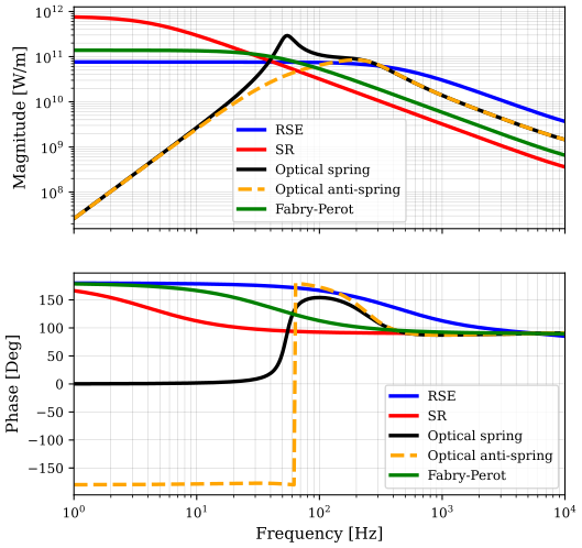
We will compute the optomechanical plant for five cases to illustrate the dynamics of
the DRFPMI using the simple DARM coupled cavity. Letting \(\phi_\mathrm{s}\) denote
the extra one-way phase the carrier accumulates when propagating through the SEC, which
is equivalent to SEM.phi, these cases are
No SEM present: this is just a single Fabry-Perot cavity which is equivalent to a gravitational wave detector without an SEC, like the initial gravitational wave detectors. If the SEM is misaligned it will not form a cavity and it is effectively absent (except it will still add loss if there was any). This is accomplished in finesse by setting
SEM.misaligned=True.Signal recycling (SR): when \(\phi_\mathrm{s}=0\), the bandwidth is narrowed and the DC gain is increased relative to the single FP cavity.
Resonant sideband extraction (RSE): when \(\phi_\mathrm{s} = \pi/2\), the bandwidth is broadened and the DC gain is reduced relative to the single FP cavity. This is how most gravitational wave detectors operate.
Optical spring: when \(\phi_\text{s}>\pi/2\), there is an anti-damped optical spring. This is how the low frequency Einstein telescope is planned to operate.
Optical anti-spring: when \(\phi_\text{s}<\pi/2\), there is a damped anti-spring.
Note that there is no standard convention and often \(\phi_\mathrm{s}\) is defined
as SEM.phi - \pi/2 in the literature and other codes so that all of the above cases
shift by \(\pi/2\).
We’ll compute the same transfer function for each of these cases and so define a simple
function fresp which returns the same frequency response giving it a different name
so that it can be retrieved easily from the solution. Then we’ll compute these five
cases in a Series using Change between each to set the
correct configuration. Since this will change the state of the model we do this in a
temporary_parameters context manager so that the model reverts back to its initial
state after the analysis.
F_Hz = np.geomspace(1, 10e3, 300)
fresp = lambda k: fa.FrequencyResponse(
    F_Hz, "ETM.mech.z", "BHD.DC", carrier_solution=DC, name=k,
)

with model.temporary_parameters():
    sol = model.run(fa.Series(
        fa.Change({"SEM.phi": 0}),
        fresp("SR"),
        fa.Change({"SEM.phi": 90}),
        fresp("RSE"),
        fa.Change({"SEM.phi": 98}),
        fresp("spring"),
        fa.Change({"SEM.phi": 82}),
        fresp("anti"),
        fa.Change({"SEM.misaligned": True}),
        fresp("arm"),
    ))
Note that detuning the arm is a situation where you would need to think carefully about
manually setting the carrier_solution. There is now an extra phase introduced in the
arm and so you would either need to retrieve the new operators with an
Operator action (the most robust) or multiply all of the fields by the
appropriate phase. There are no DC fields in the SEC so we did not need to worry about
that in this case where we only detuned the SEC.
The effective coupled cavity transfer functions need to be divided by \(\sqrt{2}\) to account for the presence of the beamsplitter in the DRFPMI.
plt_fresp = lambda k: sol[k].out.squeeze() / np.sqrt(2)
lw = 2.5
axs = bode(F_Hz, plt_fresp("RSE"), db=False, label="RSE", lw=lw)
bode(F_Hz, plt_fresp("SR"), axs=axs, db=False, label="SR", lw=lw)
bode(
    F_Hz, plt_fresp("spring"), axs=axs, db=False, label="Optical spring", lw=lw,
)
bode(
    F_Hz, plt_fresp("anti"), axs=axs, db=False, label="Optical anti-spring",
    ls="--", lw=lw,
)
bode(F_Hz, plt_fresp("arm"), axs=axs, db=False, label="Fabry-Perot", lw=lw)
axs[0].set_ylabel("Magnitude [W/m]")
Text(0, 0.5, 'Magnitude [W/m]')