Your first Finesse model

1. Mapping the Optical System

To run a simulation, you need to create a simple text describing your optical setup, simulation commands and optional comments. This can be a multi-line string in a Jupyter notebook cell, or a text file (“kat file”) that you load. Before writing any code, start by visualising and mapping the system you want to model. Sketch the optical setup and identify all major components such as lasers, mirrors, beamsplitters, free spaces, and others. Then, you must break the system down into basic components and the nodes that connect them. Nodes represent the points of connection or separation between two components. Finally, assign a short and unique name to every component. This name is how you’ll refer to the element in the input file commands and how Finesse will reference it in any output or internal messages.

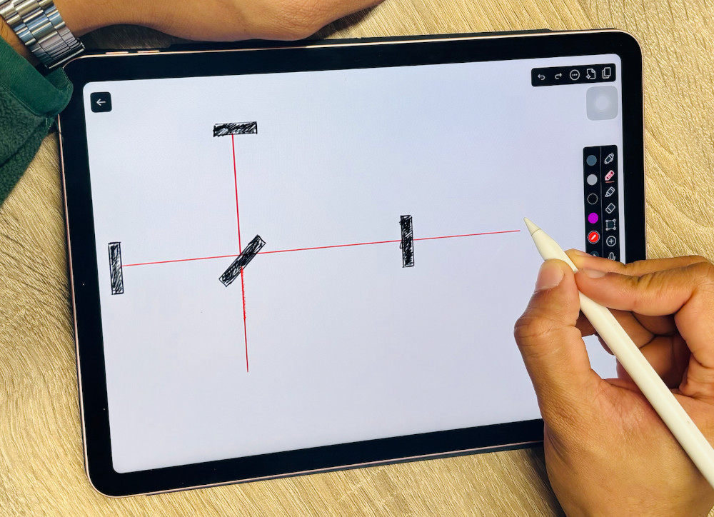
Fig. 3 Sketching a model by hand

2. Describing Components and Connections

The input file consists of a series of component descriptions and commands. We call the Finesse syntax to describe these components KatScript. A component description is typically entered on a single line following the following format:

keyword name parameters

The keyword specifies the component type (for example m for mirror, s for space, l for laser). Following the name are the parameters, which are numerical values defining the component’s properties, such as power (P), frequency (f) for a laser, or power reflectivity (R), power transmissivity (T), and tuning (phi) for a mirror.

For example, a laser named laser1 with P=1 W, zero frequency offset from the default frequency (ref), is described as:

l laser1 P=1 f=0

A mirror named mirror1 with R=0.9 and T=0.1 is described as:

m mirror1 R=0.9 T=0.1

In Finesse, connectivity is defined using ‘Ports’ and ‘Nodes’. This mechanism allows the model to handle not only the flow of light but also complex feedback loops involving electrical and mechanical signals.

Most components feature various Ports (e.g., p1, p2) which are its connection points. Each port then contains one or more ‘Nodes’ that represent the actual light or signal information flow. You access these specific states directly using the standard convention: component.port.node.

• Optical Ports always contain an Input Node (.i) and an Output Node (.o), describing the field entering and exiting the component. Optical connections between elements must be made using a Space ( component (or alternatively using the Link command).

• Electrical and Mechanical Ports contain Signal Nodes. These nodes represent small, linearised states (such as mirror motion or voltage) and are vital for modeling active control systems, as they can be connected using Wires to form feedback loops.

Most components connect to exactly two nodes. Sources, like lasers connect to one, and beam splitters connect to four. Crucially, every node must connect to at least one component but never more than two, or the system description will be inconsistent.

Detectors are special components. They can be placed at any node in the interferometer (without blocking the existing light or signal flow at that node), and each detector specifies one output variable to be computed. Specifying multiple detectors allows for the computation of several signals simultaneously.

3. Defining the Simulation Task

Commands in Finesse are primarily used to define global model properties, enabling advanced analysis features and higher-order modes (HOMs), and these are not yet necessary for your first simulations.

All simulations in Finesse are run via the Python Application Programming Interface (API). An API is essentially a set of clearly defined tools and protocols that allows your Python code to interact with and control the Finesse simulation engine. This allows for adaptable, computationally efficient analysis directly within your scripts.

All simulations are executed using Actions, which are single or multiple atomic simulation tasks that form a complete Analysis to be performed on the model. This system is efficient because the model is built only once, allowing complex analyses to be defined and run sequentially or concurrently.

The most basic simulation task is performed by the Xaxis Action. To use it, you must import the Xaxis class from finesse.analysis.actions and pass the instantiated object directly to the model.run() method. This Action sweeps a parameter, computes all detector outputs, and returns the result as a Solution object.

For example, to sweep the power of the laser (l1.P) linearly from 0 to 1 over 10 steps, you write:

from finesse.analysis.actions import Xaxis

# ... model definition here ...
sol = model.run(Xaxis(model.l1.P, 'lin', 0, 1, 10))

Finesse includes a wide range of specialized Actions and Analysis tools designed for different computational tasks, such as finding a system’s operating point, calculating noise curves, or modeling complex locking schemes. [link to finesse analysis actions]()

The next section contains a first Finesse example.