Basics of Using Maps

Introduction

In Finesse, maps are used to model spatial imperfections on optics, such as surface figure errors or refractive index variations. These maps can be applied to certain elements to simulate real-world effects like scattering, mode mismatch, or thermal lensing. They can also be used outside of a simulation environment to visualize deformations and computer mode scattering matrices.

Most of the map functionality can be found in the finesse.knm and finesse.utilities.maps modules. A prerequisite for these sections is an understanding of the section Modelling with higher-order modes.

Note

You will often see knm used in the context of maps. This is a reference to the \(K\) matrices which are often used in analytics to represent a scattering operator.

What is a Map?

A map is a 2D array that represents a spatially varying optical property, such as:

• Surface height variations (phase maps)

• Refractive index gradients (substrate maps)

• Losses (amplitude maps)

Maps modify the behavior of optical elements by changing the phase and/or amplitude of the fields interacting with them.

Supported Maps

Finesse currently supports the following types of maps:

• Surface maps: Change the optical phase on reflection; typically used to simulate surface deformations.

• Absorption maps: Describe spatially varying loss or transmission, e.g. from absorption or aperturing

• Substrate maps: Simulate index of refraction changes, e.g., from thermal lensing.

Not all optical elements support maps. The following elements can use maps:

• Mirrors: Apply surface maps to modify the phase of reflected light.

• Beamsplitters: Also apply surface maps to modify the phase of reflected light.

• Lens: Apply substrate maps to modify the phase of transmitted light.

You can typically combine the above elements to create more complex systems, like a thick distorted optic.

Coordinate system

Maps are defined in a 2D coordinate system, where the origin (0,0) is on the beam axis. The right-handed coordinate system used for the maps is shown here for mirrors and beamsplitters:

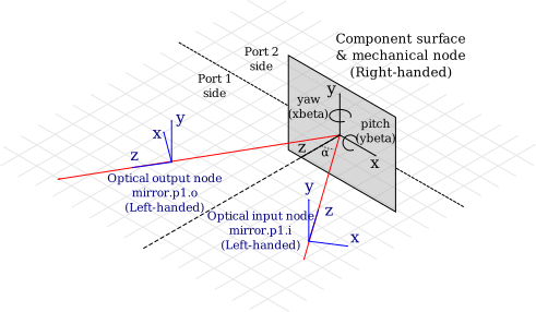
The surface normal vector is in the positive z direction for the component is important for surface deformations. A positive z value results in a ‘hill’ on the surface, a negative z value results in a ‘valley’.

For lenses the z-component does not matter. The lens OPD_map just describes an optical delay and has no directionality associated with it. The x and y directions are the same as for mirrors and beamsplitters.

Generating maps

Unlike Finesse 2.0, there is currently not a defined map file format. Instead, maps are generated at runtime using Python code.

Amplitude maps

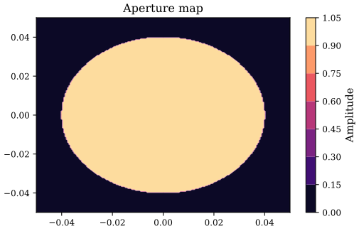
In this simple example we make a 10x10cm aperture map with a 4cm radius and a value of 1 inside the aperture and 0 outside. The value of amplitude should be between 0 and 1, although there are no checks internally in Finesse to enforce this, so be careful.

import finesse
from finesse.knm.maps import Map
import numpy as np
import matplotlib.pyplot as plt

finesse.init_plotting()

# Create a 10x10cm map
# We recommend using different number of X and Y points to avoid
# issues with transposing maps and data.
x = np.linspace(-5e-2, 5e-2, 200)
y = np.linspace(-5e-2, 5e-2, 201)

X, Y = np.meshgrid(x, y)
R = np.sqrt(X**2 + Y**2)
aperture = np.zeros((y.size, x.size))
aperture[R < 4e-2] = 1
my_map = Map(x, y, amplitude=aperture)

plt.contourf(x, y, my_map.amplitude)
plt.colorbar(label="Amplitude")
plt.title("Aperture map");

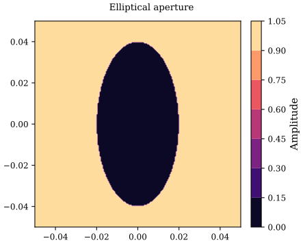
There are numerous ways to achieve this but we could also make an elliptical aperture map by changing the scale of the x and y coordinates.

R = np.sqrt((X / 0.5)**2 + Y**2)
aperture = np.ones((y.size, x.size))
aperture[R < 4e-2] = 0
my_map = Map(x, y, amplitude=aperture)

plt.contourf(x, y, my_map.amplitude)
plt.colorbar(label="Amplitude")
plt.title("Elliptical aperture")

Text(0.5, 1.0, 'Elliptical aperture')

Surface error maps

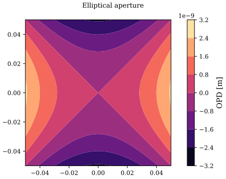
Phase maps are similar to amplitude maps, but they are used to represent optical path difference (OPD) variations relative to no map being present. The OPD must have units of meters because at this stage the map is not referenced to a particular wavelength and depends what the default model wavelength is. The phase accumulated across the wavefront is the OPD multiplied by the wavenumber \(k\):

\[\phi(x,y) = k \rm{OPD}(x,y)\]

The OPD can be set by using the opd keyword argument as seen here:

X, Y = np.meshgrid(x, y)
my_map = Map(x, y, opd=1e-6 * (X**2 - Y**2))

plt.contourf(x, y, my_map.opd)
plt.colorbar(label='OPD [m]')
plt.title("Elliptical aperture")

Text(0.5, 1.0, 'Elliptical aperture')

Generating the complex-valued map

The complex-valued map is generated by using the Map.get_z method of the map object.

\[z(x,y) = \rm{amplitude}(x,y) \exp\left( \I F k \rm{OPD}(x,y) \right)\]

Where \(F\) is the phase factor for a particular scenario. A phase map can be used to describe a surface height, or a refractive index change over the length of a substrate. Commonly used values for \(F\) are:

• 1: Substrate refractive index change map

• 2: Surface reflection (Factor of 2 for a double pass on reflection)

• \(n_{1}-n_{2}\): Transmission through a refractive index change at a surface

Finesse will apply these scaling terms internally depending on what the component is using the map for. The components documentation should be referred to for exactly how the data should be provided.

Here for example is an apertured map with some surface variation, we then plot the resulting phase map that would perturb the optical field.

X, Y = np.meshgrid(x, y)
R = np.sqrt(X**2 + Y**2)
aperture = np.ones((y.size, x.size))
aperture[R > 4e-2] = 0
k = 2*np.pi/1064e-9 # Or use model.k0 if you have a finesse model

my_map = Map(x, y, opd=1e-6 * (X**2 - Y**2), amplitude=aperture)

Z = my_map.get_z(
    k,
    2, # factor of 2 for surface reflection
)

fig, axs = plt.subplots(1, 2, figsize=(12, 5))

# Plot phase
contour1 = axs[0].contourf(x, y, np.angle(Z))
fig.colorbar(contour1, ax=axs[0], label='Phase [rad]')
axs[0].set_title('Phase')

# Plot amplitude
contour2 = axs[1].contourf(x, y, np.abs(Z))
fig.colorbar(contour2, ax=axs[1], label='Amplitude')
axs[1].set_title('Amplitude')

plt.tight_layout()

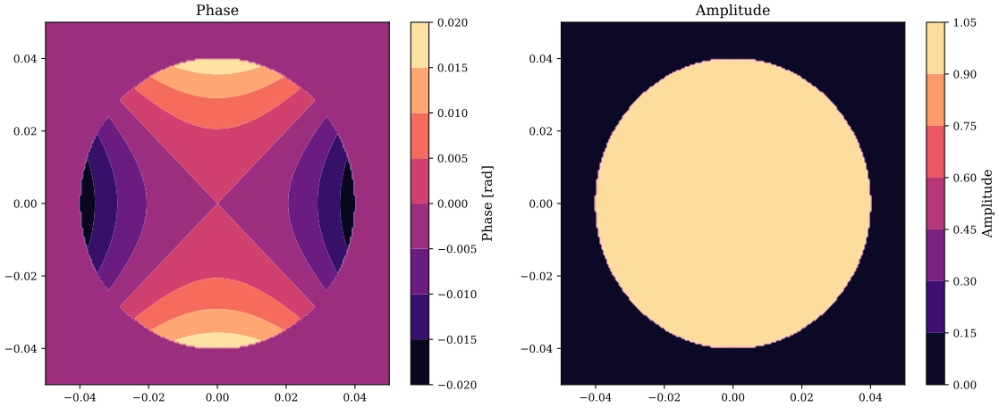
Computing scattering matrices

When performing modal model simulations the scattering matrix (or scattering operator) is typically what you are interested in. How much does one Hermite-Gaussian mode couple to another. This can be computed from the map directly for a given wavenumber, set of modes indices, and a beam parameter describing the shape of the beam at this map. Again, Finesse will apply all this information for you when it runs simulations internally, this is simply a helper method for users to experiment and see the effect of maps on the mode scattering. Below we should see that is a larger complex scattering into from the HG00 to the HG10 due to the map representing a tilted surface.

Note

See Hermite-Gauss modes and coupling for a more mathematical description of the scattering matrix and how to compute it.

X, Y = np.meshgrid(x, y)
k = 2 * np.pi / 1064e-9 # Or use model.k0 if you have a finesse model
homs = [
    (0,0), # HG00
    (1,0), # HG10
    (0,1), # HG01
]

q = finesse.BeamParam(w=2e-2, Rc=np.inf)

my_map = Map(x, y, opd=1e-9 * X)
K = my_map.scatter_matrix(
    q,
    k,
    1,
    homs,
)

display(K)
print(K)

<finesse.knm.matrix.KnmMatrix at 0x55cb420ba910>

K[0][0]: 0 0 -> 0 0 = (0.9999989944757481-1.3806581657872145e-20j)
K[1][0]: 0 0 -> 1 0 = (-3.0724160948663404e-17-5.905165798665218e-05j)
K[2][0]: 0 0 -> 0 1 = (-1.6653345369377348e-16-3.009265538105056e-36j)
K[0][1]: 1 0 -> 0 0 = (-3.0724160948663404e-17-5.905165798665218e-05j)
K[1][1]: 1 0 -> 1 0 = (0.9999858480526327-1.5357119720985648e-20j)
K[2][1]: 1 0 -> 0 1 = (4.622231866529366e-33+6.776263578034403e-21j)
K[0][2]: 0 1 -> 0 0 = (-1.6653345369377348e-16-3.009265538105056e-36j)
K[1][2]: 0 1 -> 1 0 = (4.622231866529366e-33+6.776263578034403e-21j)
K[2][2]: 0 1 -> 0 1 = (0.9999858432596216-1.3806400084350208e-20j)