Models and Components
Using the python interface to construct your Finesse model can be more verbose than using KatScript, but gives you access to syntax highlighting and autocompletion, especially when using a modern IDE like VSCode or PyCharm. It also offers the most feature rich API to interact with Finesse models. All features are supported in Python API, whereas only a subset are support in KatScript.
Note
If you want to know how to map a KatScript command to a Python method or class you
can inspect the _register_constructs method in
script/spec.py which sets up the various links between KatScript and
Python API.
Adding components to a model
All the KatScript components, have a Python class associated in either
the finesse.components or the finesse.detectors module. Documentation can
also be accessed using the python help() method
from finesse import Model
from finesse.components import Laser, Mirror, Space, Beamsplitter
from finesse.detectors import PowerDetector

# help(Laser) # would print the help for the Laser
Adding components is done using finesse.model.Model.add(), which returns the
component added.
model = Model()
l1 = model.add(Laser("l1", P=10))
l1
<'l1' @ 0x7ff419f5a270 (Laser)>
Adding a component automatically creates an attribute on the
finesse.model.Model object with the name of the component.
model.l1
<'l1' @ 0x7ff419f5a270 (Laser)>
Note
When writing a python script, your IDE might warn you that these attributes don”t
exist and not provide autocompletion. When working in an interactive/Jupyter
context, these attributes will be available for autocompletion after the add
method has been executed.
Component names need to be unique:
model = Model()
model.add(Laser("l1", P=10))
model.add(Laser("l1", P=10))
FinesseException: 	(use finesse.tb() to see the full traceback)
An element with the name l1 is already present in the model (Laser('l1', signals_only=False, f=0.0, phase=0.0, P=10.0))
The finesse.model.Model.add() function also accepts an iterable of components:
model = Model()
l1, l2, l3 = model.add([Laser(f"l{i}", P=i) for i in range(3)])
model.components
(<'l0' @ 0x7ff41918c410 (Laser)>,
 <'l1' @ 0x7ff41918c910 (Laser)>,
 <'l2' @ 0x7ff41918c690 (Laser)>)
Connecting components
For any useful simulation, components have to be connected together. Many spaces must be made in more complicated models and often you do not need to give them a name. Therefore the python interface provides multiple ways of doing so depending on your use case.
Specifying ports on Space components
Directly adding a Space element is the most low-level option. We first create and add the components for a simple cavity:
m = Model()

l1, m1, m2 = m.add(
    [Laser("l1"),
     Mirror("m1", R=0.1, T=0.9),
     Mirror("m2", R=0.1, T=0.9)
    ]
)
And then we create finesse.components.space.Space components, connecting their
ports to the ports of existing components.
s1 = m.add(Space("s1", portA=l1.p1, portB=m1.p1))
s2 = m.add(Space("s2", portA=m1.p2, portB=m2.p1))
Using the connect method
The finesse.model.Model.connect() connects the provided components or ports
together and returns the created space/wire component. It tries to connect in a “smart”
way, so it can be useful to use the verbose argument to see what is happening.
m = Model()

l1 = Laser("l1")
m1 = Mirror("m1", R=0.1, T=0.9)
m2 = Mirror("m2", R=0.1, T=0.9)

m.add([l1, m1, m2])

s1 = m.connect(l1, m1, L=1, name="s1", verbose=True)
s2 = m.connect(m1, m2, L=1, name="s2", verbose=True)
Selecting port <Port l1.p1 Type=NodeType.OPTICAL @ 0x7ff4191d61a0> for <'l1' @ 0x7ff41918d310 (Laser)>
Selecting port <Port m1.p1 Type=NodeType.OPTICAL @ 0x7ff4191d7380> for <'m1' @ 0x7ff41918d450 (Mirror)>
Selecting port <Port m1.p2 Type=NodeType.OPTICAL @ 0x7ff4191d7450> for <'m1' @ 0x7ff41918d450 (Mirror)>
Selecting port <Port m2.p1 Type=NodeType.OPTICAL @ 0x7ff4191e4050> for <'m2' @ 0x7ff41918d590 (Mirror)>
Using the link method
The finesse.model.Model.link() method calls the
finesse.model.Model.connect() method between each pair of components provided.
Connector names will be autogenerated, but it is possible to specify the length/time
delay of the connector by adding integers to the argument list. This is useful
when you have a long list of components to connect quickly.
m = Model()

l1 = Laser("l1")
m1 = Mirror("m1", R=0.1, T=0.9)
m2 = Mirror("m2", R=0.1, T=0.9)
# Connect with distances l1 - 10m -> m1 - 20m -> m2
m.link(l1, 10, m1, 20, m2, verbose=True)
Connecting l1 to m1
Selecting port <Port l1.p1 Type=NodeType.OPTICAL @ 0x7ff4191d4870> for <'l1' @ 0x7ff41918da90 (Laser)>
Selecting port <Port m1.p1 Type=NodeType.OPTICAL @ 0x7ff4191f1640> for <'m1' @ 0x7ff41918dbd0 (Mirror)>
Connecting m1 to m2
Selecting port <Port m1.p2 Type=NodeType.OPTICAL @ 0x7ff4191f1710> for <'m1' @ 0x7ff41918dbd0 (Mirror)>
Selecting port <Port m2.p1 Type=NodeType.OPTICAL @ 0x7ff4191f2270> for <'m2' @ 0x7ff41918dd10 (Mirror)>
You can also be more verbose with the ports linked m.link(l1.p1, 10,
m1.p2, m2.p1, 20, m2.p2, verbose=True). Note that when connecting through a
component you need to specify which port to in and which to go out, as seen with
m1 above.
Using the chain method
This method is documented for completeness but maybe removed later as link and connect above are used far more frequently.
The finesse.model.Model.chain() method is similar to the
finesse.model.Model.link() method. One difference is it accepts dictionaries that
specify space components, allowing for named connectors.
m = Model()
l1, m1, m2 = m.chain(
    Laser("l1"), Mirror("m1"), {"name": "s1", "L": 1}, Mirror("m2")
)
print(m.s1)
Space('s1', user_gouy_y=None, user_gouy_x=None, nr=1.0, L=1.0)
Visualizing the model
After creating and adding your components, it can be helpful to visualize your model to ensure your components are connected like you would expect. For this example we will create a simple interferometer.
m = Model()

l1 = Laser("l1")
bs = Beamsplitter("bs", R=0.5, T=0.5)
m.link(l1, bs)

ETMx = Mirror("ETMx", R=1, T=0)
m.link(bs.p3, ETMx)

ETMy = Mirror("ETMy", R=1, T=0)
m.link(bs.p2, ETMy)

signal = PowerDetector("signal", m.bs.p4.o)
m.add(signal)
<'signal' @ 0x7ff419780ad0 (PowerDetector)>
Using component_tree
We can use finesse.model.Model.component_tree() to draw a tree of the model using
ASCI characters.
print(m.component_tree())
○ l1
╰──○ bs
   ├──○ ETMy
   ╰──○ ETMx
For larger models, it can be clearer to only display a subsection of the model, by using
the root and radius arguments to select a subset of the graph.
# Only display components that are connect directly to the end mirror
print(m.component_tree("ETMx", radius=1))
○ ETMx
╰──○ bs
We can exchange some clarity with verbosity by showing the ports components are connected
to by using the show_ports argument.
print(m.component_tree(show_ports=True))
○ l1
╰──○ bs (l1.p1 ↔ bs.p1)
   ├──○ ETMy (bs.p2 ↔ ETMy.p1)
   ╰──○ ETMx (bs.p3 ↔ ETMx.p1)
We can also include the detectors in the component tree, although they are strictly speaking not components since they are not part of the optical network.
print(m.component_tree(show_detectors=True))
○ l1
╰──○ bs
   ├──○ ETMy
   ├──○ ETMx
   ╰──○ signal
Finally we can also use component_tree to visualize other networks besides
the component network, using the network_type argument:
from finesse.utilities.network_filter import NetworkType

# note you can also use 'network_type="optical"'
print(m.component_tree(m.l1.p1.o, network_type=NetworkType.OPTICAL))
○ l1.p1.o
╰──○ bs.p1.i
   ├──○ bs.p2.o
   │  ╰──○ ETMy.p1.i
   │     ├──○ ETMy.p1.o
   │     │  ╰──○ bs.p2.i
   │     │     ├──○ bs.p1.o
   │     │     │  ╰──○ l1.p1.i
   │     │     ╰──○ bs.p4.o
   │     ╰──○ ETMy.p2.o
   ╰──○ bs.p3.o
      ╰──○ ETMx.p1.i
         ├──○ ETMx.p1.o
         │  ╰──○ bs.p3.i
         ╰──○ ETMx.p2.o
Using graphviz
You can also directly visualize the The model graph by using networkx via
finesse.model.Model.plot_graph().
m.plot_graph(graphviz=False)

<Figure size 640x480 with 0 Axes>
<Figure size 640x480 with 0 Axes>
To see more information about how the optical ports are connected, you can specify the
network type optical.
m.plot_graph(network_type="optical", graphviz=False)
<Figure size 640x480 with 0 Axes>
<Figure size 640x480 with 0 Axes>
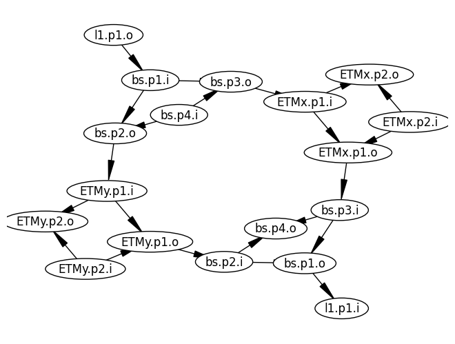
To get a prettier view, you can get use the optional pygraphviz dependency (which you should have if you used conda, otherwise see here)
m.plot_graph(network_type="optical", graphviz=True)

Note that the graphviz argument controls whether graphviz will be used. If not
available, it will automatically revert to networkx and emit a warning.
plot_graph also supports the radius and root arguments, which should be used
in tandem.
m.plot_graph(network_type="optical", graphviz=True, root="bs.p2.o", radius=2)

An alternative visualization method is finesse.model.Model.plot_dcfields_graph(), which includes the output of the finesse.analysis.actions.dc.DCFields action in the visualization:
m.plot_dcfields_graph()

PosixPath('/tmp/tmpznglsll2.svg')
Component freezing and unfreezing
Freezing and unfreezing components is a way to prevent the user from adding new
attributes of a model element accidentally. This stops the user from making commong
typos, such as setting mirror.r instead of mirror.R. The
ModelElement base class, which all components and detectors
inherit from, has a _freeze and _unfreeze method.
If the user wants to store additional attributes for a component, they can unfreeze it, set the attributes, and then freeze it again. This can be useful for storing auxiliary information about the component, such as experimental data, metadata, or other information that is not part of the model itself.
model = Model()
l1 = model.add(Laser("l1", P=10))
l1._unfreeze()
l1.my_attr = "test"
l1._freeze()
print(l1.my_attr)
test
Note
Elements are only frozen after they have been added to a model. Before that the elements are unfrozen and can be modified freely, which the user should be careful with.