Adding spatial defects with maps¶

Maps broadly speaking are 2-dimensional (x, y) information that decribes how the phase and/or amplitude of a beam is affected during some operation, such as reflection, or transmission. This is often used to decribe scenarios such as surface roughness, apertures, parametric instabiltiies, or thermal deformations. The math behind maps is described in the freely available Living Review article so will not be repeated here (See section “Scattering into higher-order modes”) [12].

Warning

Currently only mirrors and lens elements support maps - beamsplitters are a work in progress. In fact, maps in general are still a work in progress and may change in the future to fully support more options:

The map object¶

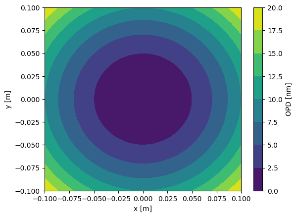
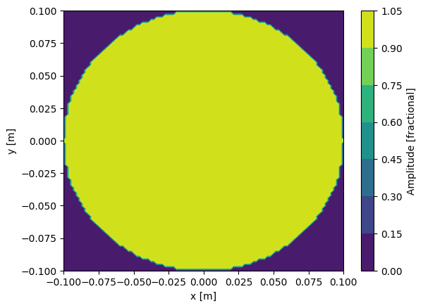
finesse.knm.Map is the object that must be created to describe a particular deformation in phase and amplitude. Below we make a simple map using a radially quadratic term and a circular aperture.

import numpy as np
import finesse
from finesse.knm import Map
from finesse.utilities.maps import circular_aperture
import matplotlib.pyplot as plt

# Always worth using a different x/y size to ensure you plot the
# correct variable later and do not transpose anything by accident
x = np.linspace(-0.1, 0.1, 100)
y = np.linspace(-0.1, 0.1, 101)
X, Y = np.meshgrid(x, y)
R = np.sqrt(X**2 + Y**2)

my_map = Map(
    x,
    y,
    opd=1e-6 * R**2,
    amplitude=circular_aperture(x, y, 0.1),
)

plt.figure()
plt.contourf(my_map.x, my_map.y, my_map.opd/1e-9)
plt.xlabel("x [m]")
plt.ylabel("y [m]")
plt.colorbar(label='OPD [nm]')

plt.figure()
plt.contourf(my_map.x, my_map.y, my_map.amplitude)
plt.xlabel("x [m]")
plt.ylabel("y [m]")
plt.colorbar(label='Amplitude [fractional]')

<matplotlib.colorbar.Colorbar at 0x7e459382b620>

This map describes the addition of some transverse quadratic phase of the beam interacting with it and will be clipped in a circular manner.

Optical path depths¶

The optical path depth (OPD) is given in units of metres and often of the order of microns or less. It should be noted that the OPD model is mostly applicable in the regime where \(OPD < \lambda\), the wavelength of the light. In cases where the OPD are signifcantly higher the number of higher order optical modes that must be used to describe the distortion can increased exponentially. This limits the application of OPDs to small perturbations to the beam that are paraxial in nature.

Quadratic lensing with maps (What not to do)¶

The simplest element to consider at first is a lens. A simple thin lens imparts a purely quadratic phase shift to a beam of the form:

\[OPD(x, y) = -\frac{1}{2 f} r^{2}\]

Where \(f\) is the focal length of the thin lens and \(r=\sqrt{x^2 + y^2}\). This is what we refer to as “quadratic lensing”.

A lens maps describe additional deformations that a beam experiences on top of the optical path depth induced by the lens itself - such as spherical aberrations or other higher order effects.

Note

Maps only work with the Python API. There is currently no methods to interact or make maps using KatScript. There are many complications in storing, inputing, and applying maps that were challenging to use in Finesse v2, none of these have been, or plan to be, implement in v3. The main limitation is that serialising a model that includes maps cannot be done at this time.

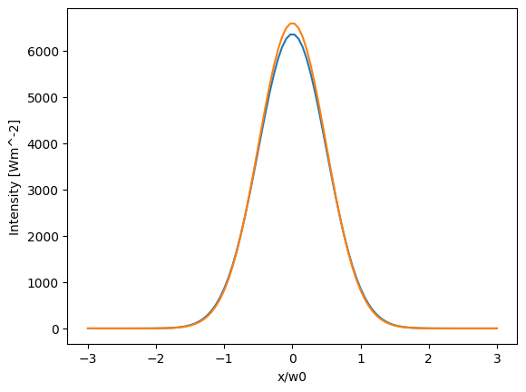
We can consider a case that is the opposite of what you should do but is somewhat illustrative: try and describe a large change in the beam shape with a map. Here we take an infinite focal length lens and apply a map that uses the \(OPD(x,y)\) above to simulate a lens with a focal length of 500m. Normally, this 500m focal length would describe a change in the beam shape using the complex beam parameter tracing (ABCD matrices and q-parameters). However now we have the situation where the q-parameters at each node are defined by the q(w0=10cm, z=0) beam through an \(f=\infty\) lens, which is the basis in which the higher order modes are described. As the map now contains the quadratic lensing the ABCD matrix knows nothing about it, so the q-parameters do not change, however to describe the fact the beam is now lensed we must include many higher order modes to describe the new shape of this lensed beam.

Below we plot a slice of the beam before and after the map is applied, we see that the beam has been focused - higher peak intensity and smaller spot size.

x = np.linspace(-0.1, 0.1, 300)
y = np.linspace(-0.1, 0.1, 301)
X, Y = np.meshgrid(x, y)
R = np.sqrt(X**2 + Y**2)
f = 500  # focal length
my_map = Map(x, y, opd=-1 / (2 * f) * R**2)

model = finesse.script.parse(
    """
                            l l
                            lens L f=inf
                            nothing n1
                            link(l, L, 10, n1)

                            gauss g1 l.p1.o w0=1e-2 z=0

                            ccdline beam n1.p1.i 100 xlim=[-3, 3]
                            modes(even, maxtem=8)
                            pd P n1.p1.i
                            """
)
out = model.run()
plt.plot(model.beam.xdata, out["beam"])
model.L.OPD_map = my_map
out = model.run()
plt.plot(model.beam.xdata, out["beam"])
plt.xlabel("x/w0")
plt.ylabel("Intensity [Wm^-2]")
print("Missing optical power:", model.l.P-out['P'], "[W]")

Missing optical power: 3.315700766171048e-06 [W]

If the map is well sampling the spot size (dx and dy are much smaller than the spot size) then you should see that using a higher maxtem will reduce the amount of power lost. There is some negligible amount lost due to the finite square aperture of the map but it should be close to a unitary transformation, so no power lost.

You can experiment yourself by trying stronger lenses and including enough higher order modes to ensure you have reached a converged state. It will often be the case with large lensing that you need exponentially more. A 100m focal length in this particular example will need maxtem > 30 to start converging.

Removing the quadratic lens¶

Altogher the correct solution here is: do not use maps to describe quadratic lensing. Higher order mode optical model using OPDs should put all the beam shaping into the ABCD beam parameters. This often results in having to “remove the quadratic term” from phase maps. This quadratic term can then be represented either in a mirror curvature or a lens focal length.

Sticking with the lens, we can do this using get_thin_lens_f. This requires specifying a spot size as well. Here our beam is 1cm. Using that we can recover what focal length the map represents.

fx = 100.5  # focal length in x
fy = 100.1  # focal length in y
my_map = Map(x, y, opd=-1 / (2 * fx) * X**2 - 1 / (2 * fy) * Y**2)
# Compute the weighted spot size focal lengths from the map OPD
my_map.get_thin_lens_f(0.01)

(np.float64(100.50000000000152), np.float64(100.1000000000015))

If you start using a beam that is perhaps to large for the map, or with a map that has spherical features (non-quadratic phase terms), then the chosen spotsize will result in different effective focal lengths. In this case it is because the beam is becoming clipped by the square aperture.

my_map.get_thin_lens_f(0.05)

(np.float64(101.49923554059183), np.float64(101.09499454289399))

Once you have retrieved and stored the quadratic terms parts then you can remove them:

original_dioptre = 1/model.L.f
new_fx, new_fy = my_map.get_thin_lens_f(0.01)
new_avg_dioptre = 1/((new_fx + new_fy)/2)
my_map.remove_curvatures(0.01, mode='average')

model.L.f = 1/(original_dioptre + new_avg_dioptre)

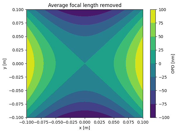
As the lens element only has a single average focal length (no astigmatic lenses yet) we have to get the average and set that to the element. Now we plot the leftover astigmatism which shouldn’t be that much, order of 10’s km.

print("New focal lengths in map:", my_map.get_thin_lens_f(0.01))

plt.figure()
plt.contourf(my_map.x, my_map.y, my_map.opd/1e-9)
plt.xlabel("x [m]")
plt.ylabel("y [m]")
plt.colorbar(label='OPD [nm]')
plt.title("Average focal length removed")

New focal lengths in map: (np.float64(-50300.25000038009), np.float64(50300.24999962069))

Text(0.5, 1.0, 'Average focal length removed')

Mirror surface maps¶

Mirror surface distortions are another common type of map we need to add. This represents a deformation to a reflective to refracting surface. The most common here is for applying residual polishing defects, or thermo-elastic deformations from thermal actuators or absorption.

The quadratic OPD of a reflecting mirror is given by:

\[OPD(x, y) = \frac{1}{4 f} r^{2}\]

Which given that \(R=2f\) is also:

\[OPD(x, y) = \frac{1}{2 Rc} r^{2}\]

Broadly similar to the lensing OPD, but there are several factors of two to consider above due to the double pass on reflection of the optic surface as well as the conversion from curvatures to focal powers. There is also a sign difference.

It is important to remember that the OPD of map for a mirror in Finesse describes the mirror surface height difference, not a total OPD (This will be fixed with a name change in a later fix). You can apply mirror surface maps using:

model = finesse.script.parse("m m1 R=0.9 T=0.1")
model.m1.surface_map = my_map

where the opd term give the Map represents the height of a surface change in the normal direction of the surface. For a mirror, a positive height change is a protrusion in the surface normal direction on the port 1 side of the element. A positive bump in the map would be a “hill” on the port 1 side, and a “valley” when seen from the port 2 side.

Quadratic mirror cuvatures terms can be calculated using finesse.knm.Map.get_radius_of_curvature_reflection. Remember that dioptes of focal length are \(\frac{1}{f}\) whereas dioptres using curvatures are \(\frac{2}{Rc}\). Mirrors have Rcx and Rcy parameters so there you can remove the quadratic astigmatic parts from maps completely.